|
|

Lotka–Volterra / Predator-Prey Simulation
Anthro-196, Tutorial #3
The Theory
The Lotka-Volterra equation models populations of predator and prey species. We start out with a few initial assumptions:
- The prey population finds ample food at all times.
- The food supply of the predator population depends entirely on the prey populations.
- The rate of change of population is proportional to its size.
- During the process, the environment does not change in favour of one species and the genetic adaptation is sufficiently slow.
So, the prey have the potential to grow unbounded since they have
infiinite food resources, while the predators can only grow while there
is an ample supply of prey to eat. The number of births and deaths of
either species increases as that species population increases. Lastly,
we ignore effects of natural selection and evolution.
Let alpha be the birth rate of the prey species and beta be the death
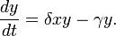
rate (Being eaten) of the prey. Let delta represent the birth rate of
the predator species and gamma be the death rate of the predators. Then
for prey species X and predator species Y, the relationship is defined
as follows:
So, the rate at which the prey species changes is equal to the number
of births minus the number eaten. The rate at which the predator
species is changing is the number of being born minus the number dying.
Notice that beta does not necessarily equal delta, so the rate at which
prey are born is not necessarily equal the number of prey being eaten.
The effect produced by running a simulation with this behavior is that
of two sine waves slightly out of phase with each other.
As the predators increase in number, the prey decrease. As the prey
population decreases, so does the population of predators that eat
them. When the predator population dips low enough, the prey population
begins to grow again. Thus, we have a cycle that continues unless the
number of predators or prey reaches zero (extinction). If the prey go
extinct, the predators will soon follow. If the predators go extinct,
than the prey will grow in population without bound.
It is also possible that the two populations will reach an equilibrium
point where the number of births and deaths cancel each other out for
both species. By solving the Lotka-Volterra equations, we find that the
equilibrium point occurs when the populations are as follows:
That is, the two populations are in equilibrium when the number of
predators is equal to the ratio of prey births to deaths and the number
of prey is equal to the ratio of predator deaths to births.
Now that you know a little bit about the theory, let's look at the simulation code.
The Code
There are two Lotka-Volterra projects. If you examine them, they
actually contain almost identical code, but running them produces very
different results. Let's look at lotka_volterra_v02 first.
This project runs a simulation based on the single-predator,
single-prey dynamics mentioned above. There are several variables
defined at the top of the file "lotka_volterra_v02.pde". The variable a
represents alpha, b beta, d delta, and g gamma. Let's try setting them
to the following values.
float x_pop= 100.0;
//population of prey
float y_pop= 20.0;
//population of predator

float z_pop= 0.0; //population of second predator

float a= 1.4;
//growthrate of prey

float b= 0.09;
//deathrate of prey, being eaten and dying

float d= 0.001;
//growthrate of predator

float g= 0.8;
//deathrate of predator

float e= 0.0;
//growthrate of second predator

float f= 0.0;
//deathrate of second predator


float t = 0;
//initial time

float t_step = 0.01;
//initial time step

float death_total = 0.0;
//initial time step

float co2_total = 0.0;
//all souls
|
Run the simulation and see what you get. The green circles represent
the prey species and the red circles represent predators. The
brightness of the color is based on the population size, so larger
populations produce brighter color intensity. You can see information
about the exact population numbers printed in the window below the
processing editor. The behaviour you should see is the oscillation
effect predicted by Lotka and Volterra. The predator population will
fluctuate between 3 and 40 members, while the prey population will
fluctuate between 90 and 2800 members.
Now, try plugging in the values for the equilibrium equation mentioned
above and set the variables x_pop and y_pop to your computed values.
(You should get 800 for x_pop and 15.556 for y_pop) You should now
observe that the predator and prey populations barely change at all.
Now go back and try changing the initial population sizes and the birht
and death rates. What kinds of behaviours do you observe? (Note that
there are some safeguards in the code to prevent either species from
going completely extinct.)
Now that you've seen the simulation running, let's take a look at the
portion of the code that actually performs the Lotka-Volterra
calculation. The code is in the lotka() function in the function.pde
file. The important bits are in red.
void lotka (){
    float x_new = 0;
    float y_new = 0;
    x_new = (a*x_pop - b*x_pop*y_pop)*t_step+x_pop;
    y_new = (d*x_new*y_pop - g*y_pop)*t_step+y_pop;
    println("from Lotka"+x_new);
    //damper

    death_total = (x_new-x_pop)+(y_new-y_pop);


    if (x_new < 1.0){
        x_pop= 1.0;
    } else {
        x_pop= x_new;
    }

    if (y_new < 1.0){
        y_pop= 1.0;
    } else {
        y_pop= y_new;
    }

    co2_total = x_pop+y_pop;

    int prey = int(x_pop/10);
    int predator = int(y_pop);

    smooth();
    for (int j = 0; j < prey; j++){
        float dia = random(25);
        fill (0, j, 0);
        ellipse(random(x_screen), random(y_screen), dia, dia);
    }
    for (int i = 0; i < predator; i++){
        float dia = random(25)+25;
        fill (i*12+128, 0, 0);
        ellipse(random(x_screen), random(y_screen), dia, dia);

    }

}
|
The first four red lines define a set of variables and set them to the
new population size for x (Prey) and y (Predator) based on the
Lotka-Volterra equation and the timestep value. Remember that the
Lotka-Volterra equation produces a rate of change over time, so we have
to multiply it by the timestep to get the actual change in population
size. The two if statements after that just keep either species from
going extinct by making sure that neither population gets too low.
Now let's take a look at lotka_volterra_v03_key. This project is very
similar to lotka_volterra_v02, except that it includes a second
predator that can eat both prey and the first predator. We now have
three equations modeled thusly:

So, the death rates of the prey and the first predator are now affected
by this new super-predator species that can eat both of them. Likewise,
the second predator's birth rate is dependant upon not only its own
population, but upon the populations of the things that it can eat.
Just as there were variables in lotka_volterra_v02 for the birth and
death rates of our original prey and predator, there are variables in
lotka_volterra_v03_key for our new species. The variable e represents
epsilon (The new predator's birth rate) and f represents zeta (The new
predator's death rate). Try the values below, then play around with the
values and see what kinds of behaviours you observe.
float x_pop= 100.0;
//population of prey
float y_pop= 20.0;
//population of predator

float z_pop= 10.0;
//population of second predator

float a= 1.4;
//growthrate of prey

float b= 0.09;
//deathrate of prey, being eaten and dying

float d= 0.001;
//growthrate of predator

float g= 0.8;
//deathrate of predator

float e= 0.0001;
//growthrate of second predator

float f= 0.9;
//deathrate of second predator


float t = 0;
//initial time

float t_step = 0.01;
//initial time step

float death_total = 0.0;
//initial time step

float co2_total = 0.0;
//all souls
|
If you would like to add some flair to your predator-prey simulation,
read on and I will show you how to replace the circles with images. We
need to make a few changes. First, we need to find some images for our
creatures and put them in the data folder of our project. Below are the
images that I used.
Prey
|
Predator 1
|
Predator 2
|
 |
 |
 |
Next, we need to load the images into our sketch. We do this by
creating a PImage variable and then calling the loadImage function in
the setup function. The lines I added are in violet. You will need to
replace the filenames with whatever your images are named. Again, make
sure your images are in the data folder!
//These lines are outside of setup()
PImage prey1;
PImage pred1;
PImage pred2;

void setup () {
  size(int(x_screen), int(y_screen));

  //These lines are inside setup()
  prey1 = loadImage("prey1_small.png");  // <--- Replace filenames!
  pred1 = loadImage("pred1_small.png");
  pred2 = loadImage("pred2_small.png");
}
|
Now in the functions.pde file, we need to locate the code that draws
the creatures and change it from drawing circles to drawing images.
I've outlined the prey's draw code in green, the first predator's draw
code in red, and the second predator's draw code in blue.
void triple_lotka (){
    float x_new = 0;
    float y_new = 0;
    float z_new = 0;
    x_new = (a*x_pop - b*x_pop*y_pop*z_pop)*t_step+x_pop;
    y_new = (d*x_new*y_pop - g*y_pop*z_pop)*t_step+y_pop;
    z_new = (e*x_new*y_new*z_pop - f*z_pop)*t_step+z_pop;
    //println("from Triple Lotka: "+z_new);
    //damper

    death_total = (x_new-x_pop)+(y_new-y_pop);


    if (x_new < 1.0){
        x_pop= 1.0;
    } else {
        x_pop= x_new;
    }

    if (y_new < 1.0){
        y_pop= 1.0;
    } else {
        y_pop= y_new;
    }

    if (z_new < 1.0){
        z_pop= 1.0;
    } else {
        z_pop= z_new;
    }

    co2_total = x_pop+y_pop;

    int prey = int(x_pop/10);
    int predator = int(y_pop);
    int predator2 = int(z_pop);
    smooth();
    for (int j = 0; j < prey; j++){
        float dia = random(25);
        fill (0, j, 0);
        ellipse(random(x_screen), random(y_screen), dia, dia);
    }
    for (int i = 0; i < predator; i++){
        float dia = random(25)+25;
        fill (i*12+128, 0, 0);
        ellipse(random(x_screen), random(y_screen), dia, dia);
    }
    for (int k = 0; k < predator2; k++){
        float dia = random(25)+25;
        fill (0, 0, (k*12)+128);
        ellipse(random(x_screen), random(y_screen), dia, dia);
    }

}
|
All that we have to do is comment out these lines and add in a few of our own.
void triple_lotka (){
    float x_new = 0;
    float y_new = 0;
    float z_new = 0;
    x_new = (a*x_pop - b*x_pop*y_pop*z_pop)*t_step+x_pop;
    y_new = (d*x_new*y_pop - g*y_pop*z_pop)*t_step+y_pop;
    z_new = (e*x_new*y_new*z_pop - f*z_pop)*t_step+z_pop;
    //println("from Triple Lotka: "+z_new);
    //damper

    death_total = (x_new-x_pop)+(y_new-y_pop);


    if (x_new < 1.0){
        x_pop= 1.0;
    } else {
        x_pop= x_new;
    }

    if (y_new < 1.0){
        y_pop= 1.0;
    } else {
        y_pop= y_new;
    }

    if (z_new < 1.0){
        z_pop= 1.0;
    } else {
        z_pop= z_new;
    }

    co2_total = x_pop+y_pop;

    int prey = int(x_pop/10);
    int predator = int(y_pop);
    int predator2 = int(z_pop);
    smooth();
    for (int j = 0; j < prey; j++){
        //float dia = random(25);
        //fill (0, j, 0);
        //ellipse(random(x_screen), random(y_screen), dia, dia);
        image(prey1, random(x_screen), random(y_screen));
    }
    for (int i = 0; i < predator; i++){
        //float dia = random(25)+25;
        //fill (i*12+128, 0, 0);
        //ellipse(random(x_screen), random(y_screen), dia, dia);
        image(pred1, random(x_screen), random(y_screen));
    }
    for (int k = 0; k < predator2; k++){
        //float dia = random(25)+25;
        //fill (0, 0, (k*12)+128);
        //ellipse(random(x_screen), random(y_screen), dia, dia);
        image(pred2, random(x_screen), random(y_screen));
    }

}
|
And that's it! You should now have pretty sharks and fish swimming around. Have fun with your simulation.

All information comes from the Wikipedia article. Wile E. Coyote and the Road Runner are properties of Warner Bros. Entertainment. No animals were harmed in the creation of this tutorial.
|
|
|